CR3BP Propagator Class in Python | Orbital Mechanics with Python 54
In this video we put everything together that we’ve gone over in the last 3 videos to create the CR3BP propagator class in Python, solve the differential equations of motion, and plug in some initial conditions in 2 and 3 dimensions that produce some very interesting trajectories.
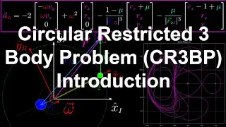
We’ll start with a use case of the CR3BP class, which is the plot creating 5 CR3BP orbits, each with the initial conditions of the 5 Lagrange points with their x-position slightly modified, and then we’ll go over the CR3BP class implementation.
Now for the CR3BP class, we start with the constructor which only takes in 1 argument which is the system. Next is the differential equation method, which like the Spacecraft class takes in the simulation time and state, and outputs the derivative of the state.
Then we have the propagate orbit method, which is where its different from the Spacecraft class (if you’ve seen that implementation on this channel and GitHub repository). In the spacecraft class, we are modeling one spacecraft per instance of the class, therefore the propagate orbit is just called in the constructor because there is nothing to modify.
But in this CR3BP class, in the constructor we only define what system the instance is modeling, and we can propagate as many orbits as we want with this instance, which is exactly whats happening in the 5 Lagrange points script, we just keep calling the cr3bp.propagate_orbits method.
Finally for the unit tests, one way to test the differential equation implementation is to plug in known periodic orbits in the CR3BP and assert that the initial state you passed in and the final state are equal to some tolerance.
In the next video we’ll be going over the derivation of the lagrange points, which occur when the velocity and acceleration of the spacecraft are equal to zero in the rotating reference frame, which occurs when the gradient of the pseudo-potential function is equal to zero. The co-linear lagrange points actually need to be solved for using a root solver method, where we have 4 equations (2 of them are redundant, giving us 3 co-linear lagrange points), where we see the 3 solutions on the plot on the top right.
#3bodyproblem #CR3BP #Python


![PUMPKINAT0R | Reason 2 Die [REMIX]](https://images.mixrolikus.cc/video/dkQtOCyWSCg)